y <- stats::rnorm(n = 100, mean = params$mean, sd = 1 / sqrt(params$prec))
cens_data <-
tibble(
i = seq_along(y),
y_true = y,
is_obs = y > 0,
y_obs = ifelse(is_obs, y, 0)
)Tl;dr
Tl;dr
One can specify non-standard distributions in JAGS by writing a likelihood as a parameter of a Bernoulli distribution. That is,
data {
  # Ones Trick
  z = rep(1, n)
  C = 10000
}
model {
  # Likelihood
  for (i in 1:n) {
    z[i] ~ dbern(L[i] / C)

    L[i] = ...
  }
}
Tobit Model
JAGS is great for quick results from some Markov chain Monte-Carlo (MCMC) algorithm, but what if we want to model data using a non-standard distribution? To this effect, assume we have data arising from a left-censored Tobit model, that is any observations less than zero are censored at zero.
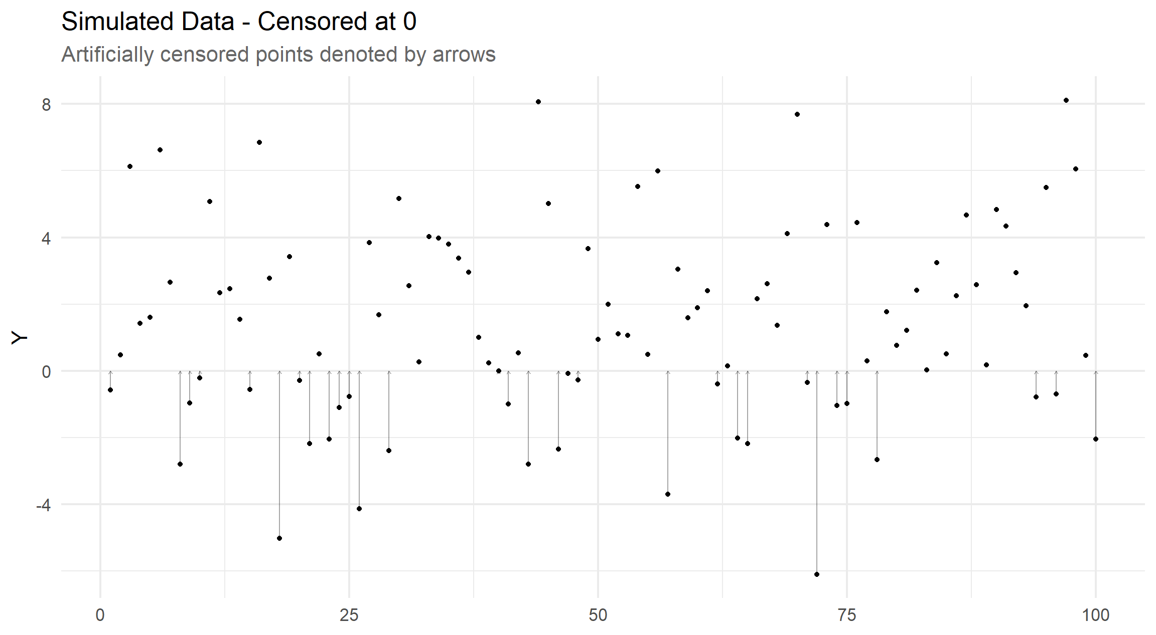
Keeping things simple, we simulate from a normal distribution (with mean equal to 1.2 and precision equal to 0.1) and then artificially censor at \(y = 0\).
In practise, we would only observe y_obs and is_obs and we keep y_true for demonstration purposes only, these data are unavailable at the modelling stage.
By convention with left-censored data, let y_obs either represents an uncensored observation, when is_obs is true, or some detection limit (in this case, 0) when is_obs is false.
The visualisation below shows how far each point is censored, if at all, and shows a 31% degree of censoring.
Likelihood
To specify a non-standard distribution, we need to be able to write down the likelihood in terms that JAGS supports.
Each contribution to the likelihood in a Tobit model is equal to either the probability density function, \(f(y_i | \mu, \tau)\), for observed (non-censored) data, or the cumulative distribution function, \(F(y_i | \mu, \tau)\), for censored data. That is, if we let is_obs[i] be denoted by \(I(y_i)\) taking the value of 1 for observed and 0 for censored data,
\[ L(\mu, \tau) = \prod_{i=1}^n f(y_i | \mu, \tau)^{I(y_i)} F(y_i | \mu, \tau)^{1 - I(y_i)} . \]
As in JAGS, we parameterise by the mean, \(\mu\), and precision \(\tau\). We use the built-in dnorm and pnorm JAGS functions for \(f\) and \(F\) respectively.
To calculate the likelihood in JAGS, assuming we have y and is_obs passed as data, we use the following
for (i in 1:n) {
  L[i] = ifelse(is_obs[i], y_pdf[i], y_cdf[i])

  y_pdf[i] = dnorm(y[i], mean, prec)
  y_cdf[i] = pnorm(y[i], mean, prec)
}
Ones Trick
Explanation
The idea of the ones trick is to assume that we have data \(z_i = 1\) for all \(i\) and then model this variable as a Bernoulli with probability \(\pi_i\). Then set this probability equal to some value proportional to the desired likelihood to effectively model the chosen likelihood in JAGS.
In general, the probability mass function of each \(z_i\) would be
\[ Pr(z_i = k_i) = \begin{cases} \pi_i, & \mathrm{if} \,\, k_i = 1, \\ 1 - \pi_i, & \mathrm{otherwise}. \end{cases} \]
The likelihood of these parameters, \(\pi = (\pi_1, \dots, \pi_n)\), would be
\[ L(\pi) = \prod_{i=1}^n \pi_i^{z_i} \, (1 - \pi_i)^{1 - z_i} . \]
Therefore, for the special case where all \(z_i = 1\) and we set the probabilities proportional to the desired likelihood from the previous section,
\[ \pi_i \propto L_i(\mu, \tau) = \frac{L_i(\mu, \tau)}{C} . \] Then the new likelihood (of \(z_i\)) is proportional to the desired likelihood (of \(y_i\)).
\[\begin{align*} L(\pi) &= \prod_{i=1}^n \frac{L_i(\mu, \tau)}{C} \\ &= \frac{1}{C} \prod_{i=1}^n L_i(\mu, \tau) \\ &\propto L(\mu, \tau) . \end{align*}\]
Warning
\(C\) is an arbitrary constant and can be set \(C = 1\), however JAGS will fail if the \(\pi_i\) exceeds one.
So a likelihood greater than one (e.g. dnorm(x = 0, mean = 0, sd = 1e-2)) would causes issues that can be avoided by setting \(C = 10000\)
Implementation
Hence the complete JAGS code is as follows, using the data block to make the call in R require no extra data.
bayestobit-univ.jags
data {
  n = length(y)

  # Ones Trick
  z = rep(1, n)
  C = 10000
}
model {
  # Likelihood
  for (i in 1:n) {
    z[i] ~ dbern(L[i] / C)

    L[i] = ifelse(is_obs[i], y_pdf[i], y_cdf[i])
    y_pdf[i] = dnorm(y[i], mean, prec)
    y_cdf[i] = pnorm(y[i], mean, prec)
  }

  # Prior
  mean ~ dnorm(0, 0.1)
  prec ~ dgamma(1, 1)
}
Simulated Example
To see this in action, we use the censored data shown earlier.
One can fit this in JAGS in their own preferred way (via jags.model then either coda.samples or jags.samples) but I am using an under development package mcmcrutils to fit this all in one go.
Tobit Model
tobit_fit <-
  mcmcrutils::complete_jags_fit(
    file = "bayestobit-univ.jags",
    data = with(cens_data, list(y = y_obs, is_obs = is_obs)),
    varnames = c("mean", "prec"),

    # Runs for 30k samples (20k discarded)
    jags_n = modifyList(mcmcrutils::jags_n_short, list(n.chains = 6)),

    # Set seed per chain (removes randomisation from re-running blog post)
    inits = inits
  )
Linear Model
For comparison, we can take a look at a similar fit that models all data as observed by imputing censored observations with half of the detection limit (in the case of a 0 detection limit, this is obviously 0).
JAGS Code for this model.
bayeslm-univ.jags
data {
  n = dim(y)
}
model {
  # Likelihood
  for (i in 1:n) {
    y[i] ~ dnorm(mean, prec)
  }

  # Prior
  mean ~ dnorm(0, 0.1)
  prec ~ dgamma(1, 1)
}
lm_fit <-
mcmcrutils::complete_jags_fit(
file = "bayeslm-univ.jags",
data = with(cens_data, list(y = ifelse(is_obs, y_obs, y_obs / 2))),
varnames = c("mean", "prec"),
# Runs for 30k samples (20k discarded)
jags_n = modifyList(mcmcrutils::jags_n_short, list(n.chains = 6)),
# Set seed per chain (removes randomisation from re-running blog post)
inits = inits
)Results
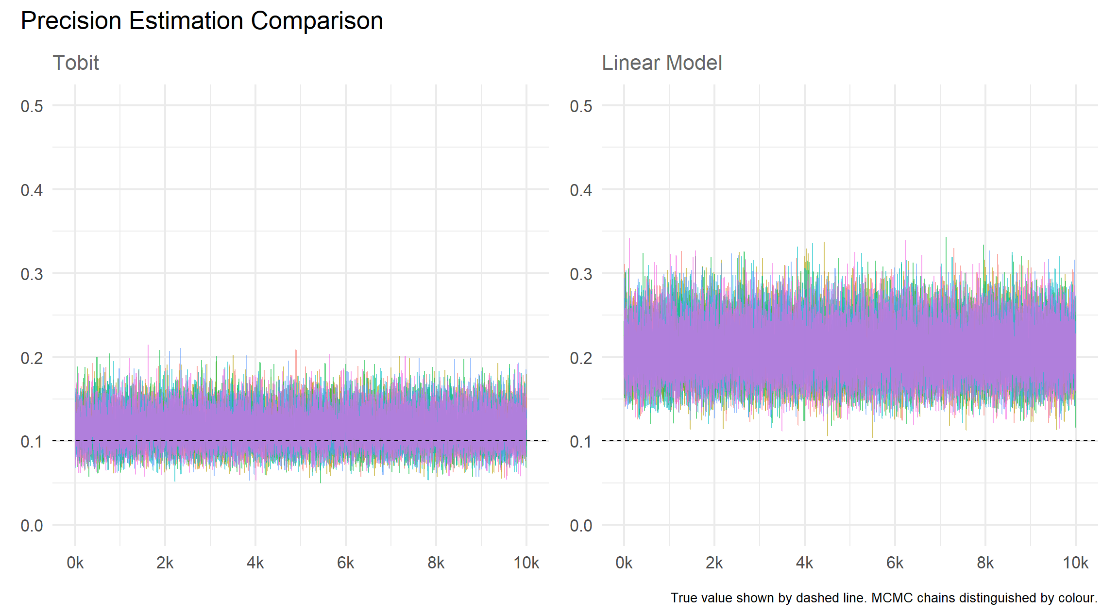
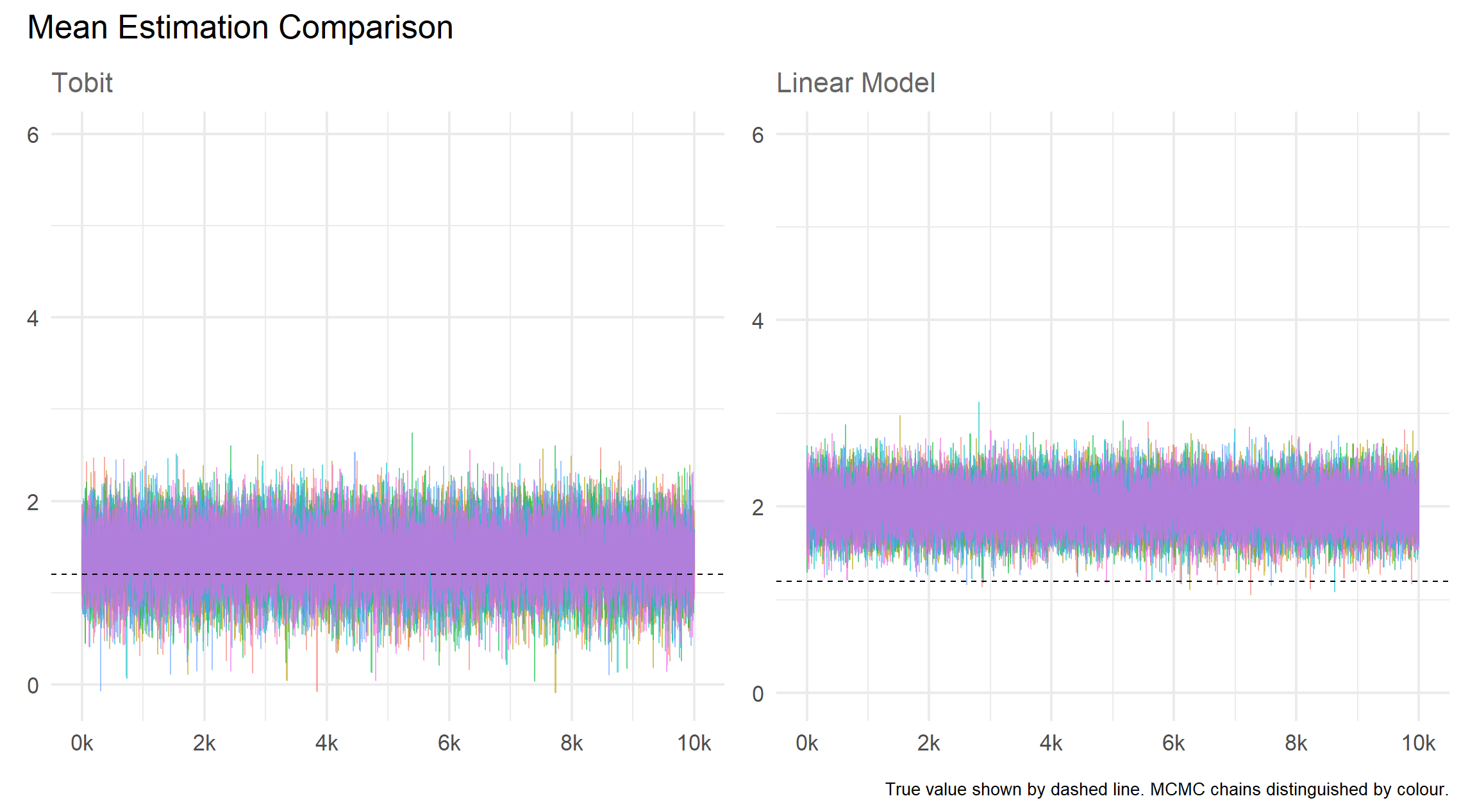
Mean
Precision