Time Series Visualisation with gghighlight and Shiny - Part 2

In the previous post, I showed how the gghighlight package can allow the showing of many time series in the background whilst focusing on a handful of selected series. Can this idea be extended with interactivity?

ggplot2
shiny
Author

Josh Cowley

Published

October 27, 2022

Tl;dr

Updating a plot by click events on the same plot is not as straightforward as one would imagine and we must save clicks in a buffer.

For the advanced Shiny user, see the app at app-current/.

Basic Setup

Recall we can simulate data from the simulate_correlated_normal function, this method is made available again but is only called once at the start of the server function.

ts_data <-
  simulate_correlated_normal(...) %>%
  tibble::rowid_to_column() %>%
  tidyr::pivot_longer(-.data$rowid) %>%
  dplyr::mutate(selected_ = FALSE)

We make a slight change to the visualisation method since the data wrangling done at the start of function was causing some issues with Shiny’s nearpoints method.

app-current/ggplot_ts.R
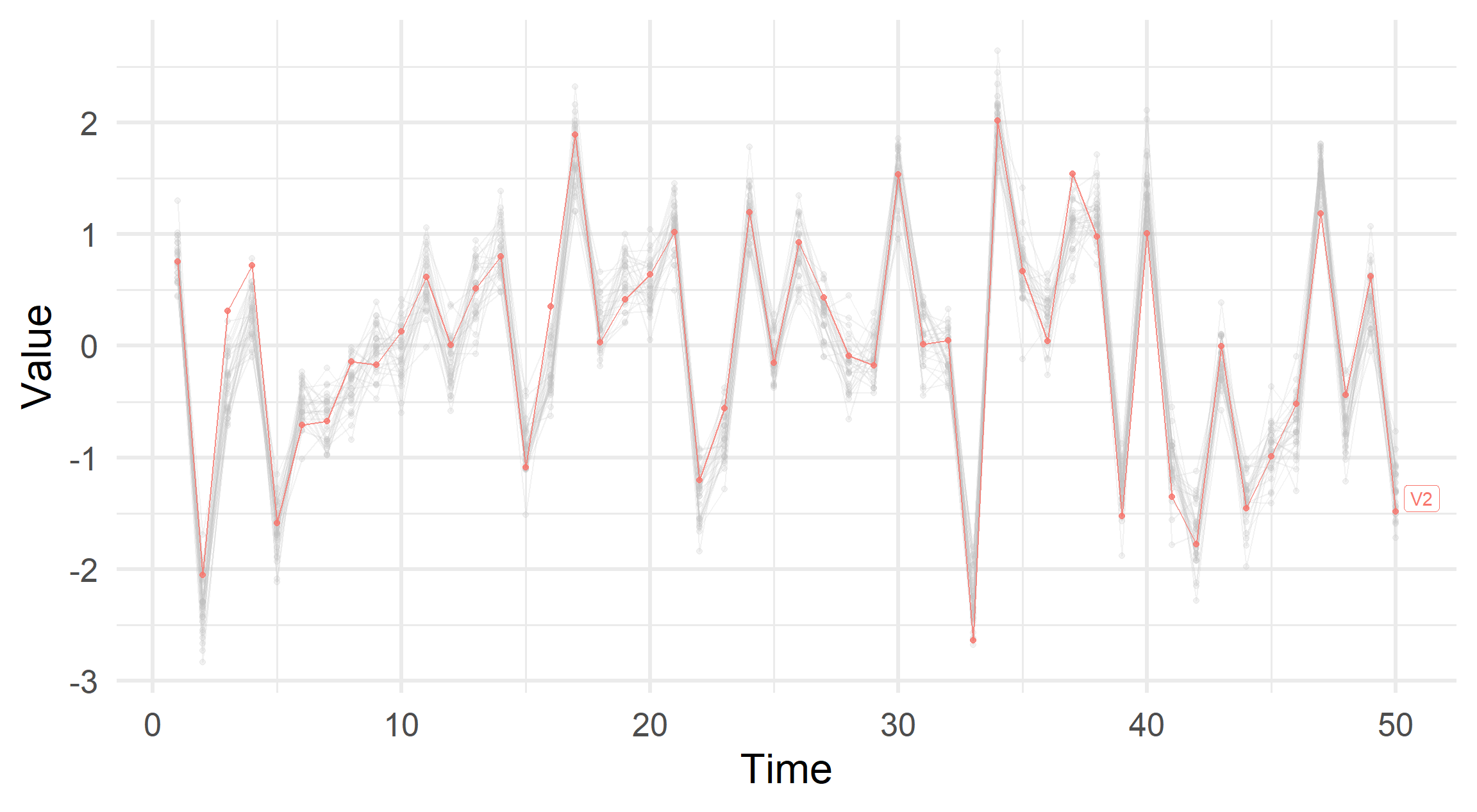
#' Visualise Time-Series Data
#' 
#' Plot used in blog post to show many time-series like data.
#' 
#' @param plot_data .
#' @param highlight character vector. Names of variables to highlight.
ggplot_ts <- function(plot_data, highlight = NULL) {
  out <- 
    plot_data %>%
    ggplot2::ggplot(ggplot2::aes(
      x = rowid,
      y = value,
      colour = name
    )) +
    ggplot2::geom_line(alpha = 0.8) +
    ggplot2::geom_point(alpha = 0.8) +
    ggplot2::labs(x = "Time", y = "Value", colour = "Series") +
    ggplot2::guides(colour = "none")
  
  if (is.null(highlight)) return(out)
  
  out +
    gghighlight::gghighlight(
      .data$name %in% highlight,
      unhighlighted_params = ggplot2::aes(alpha = 0.2),
      use_group_by = FALSE
    )
}

App 1 - Naive Attempt

The goal is simply to render a plot using the ggplot_ts function and update one of its arguments when the plot is clicked on.

To achieve this on a static plot in Shiny is straightforward, supply an ID in the UI section of the app:

shiny::plotOutput("plot", click = "plot_click")

And then the click information is available via input$plot_click in the server side of the app. It typically looks like this.

$x
[1] 2.296508

$y
[1] 0.8685864

$coords_css
$coords_css$x
[1] 157.1167

$coords_css$y
[1] 155


$coords_img
$coords_img$x
[1] 177.5418

$coords_img$y
[1] 175.15

... (etc.)

But, instead of working with this directly we can use the following to get a subset of the plot data (allRows = FALSE) or the entire data with a convenient column named selected_ (allRows = TRUE).

shiny::nearPoints(df, input$plot_click, maxpoints = 1, allRows = FALSE)

The issue arises that if we use this click information to update the plot. Then:

  1. the click information is updated by a user click,

  2. the plot updates via a defined action based on the click data,

  3. the plot re-renders and causes the user click information to reset to NULL,

  4. since the click information has changed the plot renders an erroneous second time, resetting to its original state.

To see this in action, run the following reprex where the click information and plot changes (the legend) are cleared almost instantly.

app-naive/app-naive.R
library(shiny)

ui <- 
  fluidPage(plotOutput("plot", click = "plot_click"), verbatimTextOutput("info"))

server <-
  function(input, output, server) {
    output$plot <- 
      renderPlot({
        ggplot2::qplot(
          mtcars$mpg,
          mtcars$hp,
          colour = is.null(input$plot_click)
        )
      })
    
    output$info <- renderPrint(input$plot_click)
  }

shinyApp(ui, server)

App 2 - Storing Click(s)

A workaround, using somewhat deprecated and old code is described here. We can implement this too by defining a reactiveValues object.

app-stored/app-stored.R
library(shiny)

ui <- 
  fluidPage(plotOutput("plot", click = "plot_click"), verbatimTextOutput("info"))

server <-
  function(input, output, server) {
    saved_events <- reactiveValues(plot_click = NULL)
    
    bindEvent(
      observe({saved_events$plot_click <- input$plot_click}),
      input$plot_click
    )
    
    output$plot <- 
      renderPlot({
        ggplot2::qplot(
          mtcars$mpg,
          mtcars$hp,
          colour = is.null(saved_events$plot_click)
        )
      })
    
    output$info <- renderPrint(saved_events$plot_click)
  }

shinyApp(ui, server)

This works as we store the click information in a buffer accessible by save_events$plot_click.

saved_events <- reactiveValues(plot_click = NULL)

This is then updated by an observer within bindEvent. You can think of the syntax bindEvent(observe({ x }), ...) as run { x } whenever one of the events in ... is triggered.

By using this buffer the reflection where a plot update will update click information is removed and only a click will update this buffer.

gghighlight

Issue

Back to the example at hand, extra care has to be given with gghighlight since it modifies the underlying plot object.

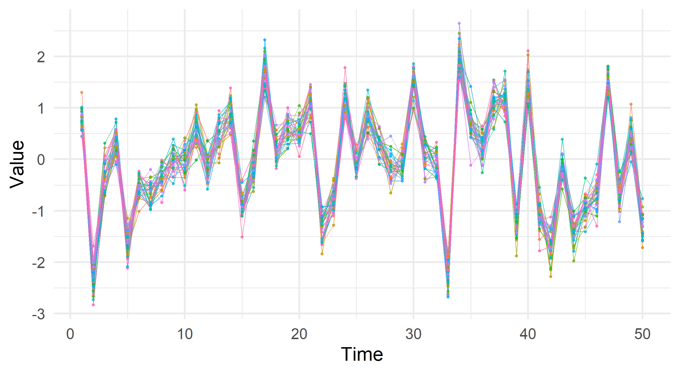
In the current iteration of the app, we start with some time series data,

ts_data <-
  simulate_correlated_normal() %>%
  tibble::rowid_to_column() %>%
  tidyr::pivot_longer(-.data$rowid) %>%
  dplyr::mutate(selected_ = FALSE)

print(head(ts_data, 5))
# A tibble: 5 x 4
  rowid name  value selected_
  <int> <chr> <dbl> <lgl>    
1     1 V1    0.853 FALSE    
2     1 V2    0.753 FALSE    
3     1 V3    0.764 FALSE    
4     1 V4    0.608 FALSE    
5     1 V5    0.576 FALSE    

And when no clicks have occurred, the plot is created via

p1 <- ggplot_ts(ts_data, NULL)

and we see this object and the default mapping for each layer:

p1
p1$mapping

Aesthetic mapping: 
* `x`      -> `rowid`
* `y`      -> `value`
* `colour` -> `name`


We can obtain the series name closest to a click using the following, where nearPoints guesses the x-axis and y-axis variables.

tb <- shiny::nearPoints(ts_data, input$plot_click, maxpoints = 1)
nm <- if (NROW(tb)) tb$name else NULL

Updating the plot is then straightforward, but the mapping for the first layer has been altered.

p2 <- ggplot_ts(ts_data, "V2")
p2
p2$layers[[1]]$mapping

Aesthetic mapping: 
* `x`      -> `highlight..........1`
* `y`      -> `highlight..........2`
* `colour` -> `highlight..........3`
* `fill`   -> NULL
* `group`  -> `highlight..........group`

This (or some other difference between p1 and p2) means that any subsequent clicks will be looking for highlight..........1 within the original data which clearly doesn’t exist and the app will crash.

Solution

The solution to this is simple (after hours of finding trial and error!). We pass the x and y names explicitly in the nearPoints call:

tb <- shiny::nearPoints(..., xvar = "rowid", yvar = "value")
nm <- if (NROW(tb)) tb$name else NULL

App 3 - Final Version

For the final version, I added some new features.

  1. Instead of a hidden buffer, store the selected series in a dropdown (selectInput) that can be changed by the user or by a click.

  2. Simulate two datasets and highlight both series in sync.

Hence, the UI file is relatively simple for demonstration purposes, just two plots alongside a dropdown input.

app-current/ui.R
ui <-
  shiny::fluidPage(
    # Sidebar panel
    shiny::sidebarPanel(
      shiny::selectInput(
        "dropdown", "Selected", choices = c("None", unique(ts_data$name))
      ),
      width = 2
    ),
    
    # Main panel
    shiny::mainPanel(
      shiny::plotOutput("plot1", click = "plot_click"),
      shiny::plotOutput("plot2"),
      width = 10
    )
  )

The server file loads the required functions, simulates two datasets and then implements what has been shown in this blog post within the server function.

app-current/server.R
library(ggplot2)
library(shiny)
library(dplyr) # %>%

source("simulate_correlated_normal.R")
source("ggplot_ts.R")

# Data to be clicked on
ts_data1 <-
  simulate_correlated_normal(offdiag = 0.2) %>%
  tibble::rowid_to_column() %>%
  tidyr::pivot_longer(-.data$rowid) %>%
  dplyr::mutate(selected_ = FALSE)

# Alternate data set
ts_data2 <-
  simulate_correlated_normal(offdiag = 0.8) %>%
  tibble::rowid_to_column() %>%
  tidyr::pivot_longer(-.data$rowid) %>%
  dplyr::mutate(selected_ = FALSE)

server <- function(input, output, session) {
  highlight <- 
    shiny::reactive(if (input$dropdown == "None") NULL else input$dropdown)
  
  shiny::bindEvent(
    shiny::observe({
      tb <- shiny::nearPoints(
        ts_data1,
        input$plot_click,
        maxpoints = 1,
        threshold = 20,
        xvar = "rowid",
        yvar = "value"
      )
      nm <- if (NROW(tb)) tb$name else NULL
      shiny::updateSelectInput(inputId = "dropdown", selected = nm)
    }),
    input$plot_click
  )
  
  output$plot1 <- shiny::renderPlot(ggplot_ts(ts_data1, highlight()))
  output$plot2 <- shiny::renderPlot(ggplot_ts(ts_data2, highlight()))
}

Further Work

Only one of the two plots change the series when clicked since nearPoints needs to know which dataset it is working on. The extension to 2 is straightforward but we would ideally have this work for any number of plots.

Shiny modules could allow this extension by using namespaces. Also modules also allow for functionality to be

  • isolated for testing,

  • re-used multiple times in the same app,

  • more easily shared.

Image Credit

Josh Cowley. October 25th, 2022. “Quayside Stone Sculptures, Newcastle Upon Tyne”.